(df <- SLD(fac=3, lev=2))Ternary plots and mixture experiments
Cornell (2002) describes a mixture experiment in which three components — polyethylene (x1), polystyrene (x2), and polypropylene (x3) — were blended to form fiber that will be spun into yarn for draperies. The response variable of interest is yarn failure load in kilograms of force applied.

The experiment is designed in a Simple Lattice Design, i.e. a regular grid of experimental points covering the whole range of possible mixtures. In R, we can create such a grid with the mixexp::SLD() function:
| x1 | x2 | x3 |
|---|---|---|
| 1.0 | 0.0 | 0.0 |
| 0.5 | 0.5 | 0.0 |
| 0.0 | 1.0 | 0.0 |
| 0.5 | 0.0 | 0.5 |
| 0.0 | 0.5 | 0.5 |
| 0.0 | 0.0 | 1.0 |
We can visualize these points on a ternary plot:
par(mar=rep(0, 4))
TernaryPlot(atip="PE", btip="PS", ctip="PP")
TernaryPoints(df, pch=16)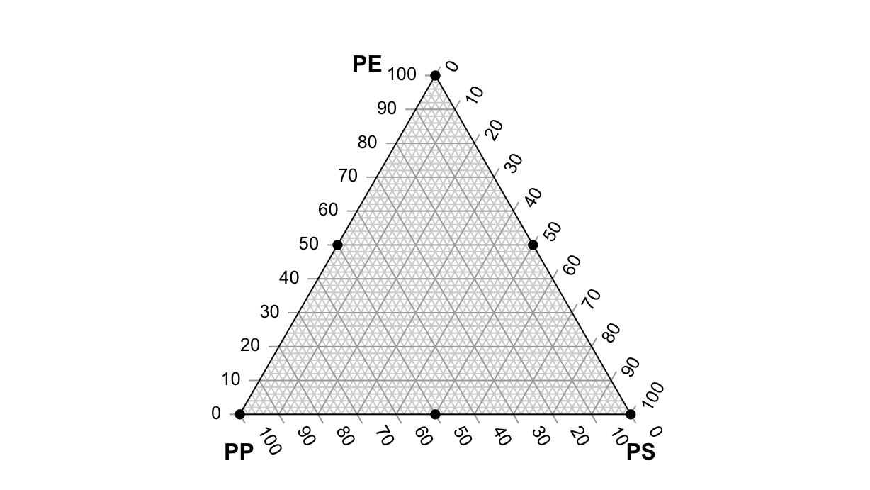
The experiments are repeated twice on corner points, thrice on mid-points. The results are:
| x1 | x2 | x3 | rep | failure |
|---|---|---|---|---|
| 1.0 | 0.0 | 0.0 | 1 | 11.0 |
| 0.5 | 0.5 | 0.0 | 1 | 15.0 |
| 0.0 | 1.0 | 0.0 | 1 | 8.8 |
| 0.5 | 0.0 | 0.5 | 1 | 10.0 |
| 0.0 | 0.5 | 0.5 | 1 | 16.8 |
| 0.0 | 0.0 | 1.0 | 1 | 17.7 |
| 1.0 | 0.0 | 0.0 | 2 | 12.4 |
| 0.5 | 0.5 | 0.0 | 2 | 14.8 |
| 0.0 | 1.0 | 0.0 | 2 | 10.0 |
| 0.5 | 0.0 | 0.5 | 2 | 9.7 |
| 0.0 | 0.5 | 0.5 | 2 | 16.0 |
| 0.0 | 0.0 | 1.0 | 2 | 16.4 |
| 0.5 | 0.5 | 0.0 | 3 | 16.1 |
| 0.0 | 0.5 | 0.5 | 3 | 11.8 |
| 0.5 | 0.0 | 0.5 | 3 | 16.6 |
We can fit a linear model to the data. On mixture experiments, the grand mean term shall be removed from the fitting formula, since at leas one factor is always non-zero (note the -1 term in the formula):
lm(failure ~ x1 * x2 * x3 - 1, data=df) %>% summary()
Call:
lm(formula = failure ~ x1 * x2 * x3 - 1, data = df)

Residuals:
   Min     1Q Median     3Q    Max
-3.067 -0.675 -0.300  0.750  4.500

Coefficients: (1 not defined because of singularities)
         Estimate Std. Error t value Pr(>|t|)
x1         11.700      1.639   7.137 5.44e-05 ***
x2          9.400      1.639   5.734 0.000282 ***
x3         17.050      1.639  10.401 2.58e-06 ***
x1:x2      19.000      7.083   2.683 0.025098 *
x1:x3      -9.100      7.083  -1.285 0.230929
x2:x3       6.567      7.083   0.927 0.378039
x1:x2:x3       NA         NA      NA       NA
---
Signif. codes:  0 '***' 0.001 '**' 0.01 '*' 0.05 '.' 0.1 ' ' 1

Residual standard error: 2.318 on 9 degrees of freedom
Multiple R-squared:  0.9832,    Adjusted R-squared:  0.9721
F-statistic: 87.96 on 6 and 9 DF,  p-value: 1.78e-07
We can improve the model by removing the interactions x1:x3, x2:x3, and x1:x2:x3:
df.lm <- lm(failure ~ x1 * x2 * x3 - 1 - x1:x2:x3 - x1:x3 - x2:x3, data=df)
df.lm %>% summary()
Call:
lm(formula = failure ~ x1 * x2 * x3 - 1 - x1:x2:x3 - x1:x3 -
    x2:x3, data = df)

Residuals:
   Min     1Q Median     3Q    Max
-3.973 -1.028 -0.300  1.377  3.209

Coefficients:
      Estimate Std. Error t value Pr(>|t|)
x1      10.520      1.518   6.930 2.49e-05 ***
x2      10.356      1.518   6.822 2.87e-05 ***
x3      16.826      1.387  12.133 1.04e-07 ***
x1:x2   19.447      7.161   2.716   0.0201 *
---
Signif. codes:  0 '***' 0.001 '**' 0.01 '*' 0.05 '.' 0.1 ' ' 1

Residual standard error: 2.438 on 11 degrees of freedom
Multiple R-squared:  0.9773,    Adjusted R-squared:  0.9691
F-statistic: 118.6 on 4 and 11 DF,  p-value: 5.743e-09
Now we can make a contour plot of the model on the ternary domain. To do that, we need to create a function representing the regressed model:
failure <- function(a, b, c) predict(df.lm, newdata=data.frame(x1=a, x2=b, x3=c))With this function we can create the plot:
par(mar=rep(0, 4))
TernaryPlot(atip="A", btip="B", ctip="C", grid.minor.lines = 1)
TernaryContour(failure, filled=T)
TernaryPoints(df %>% select(x1:x3), cex=scales::rescale(df$y, to=c(0.5, 2)), pch=16)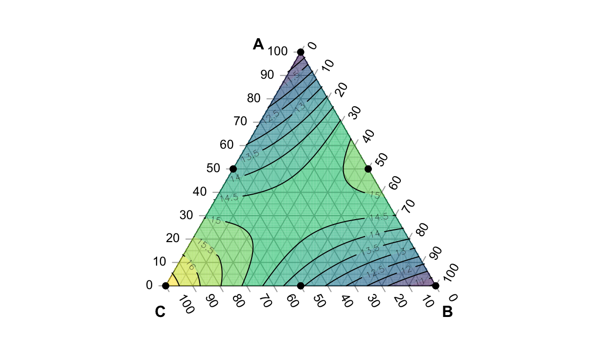
Constrained mixture space
Suppose that we have constraints on the mixture. We can create a centered design with mixexp::Xvert():
df <- Xvert(
  nfac = 3,
  lc = c(5, 25, 30)/100,
  uc = c(35, 90, 80)/100,
  plot = FALSE,
  ndm  = 1
)

par(mar=rep(0, 4))
TernaryPlot(atip="PE", btip="PS", ctip="PP")
TernaryPoints(df %>% select(x1:x3), pch=16)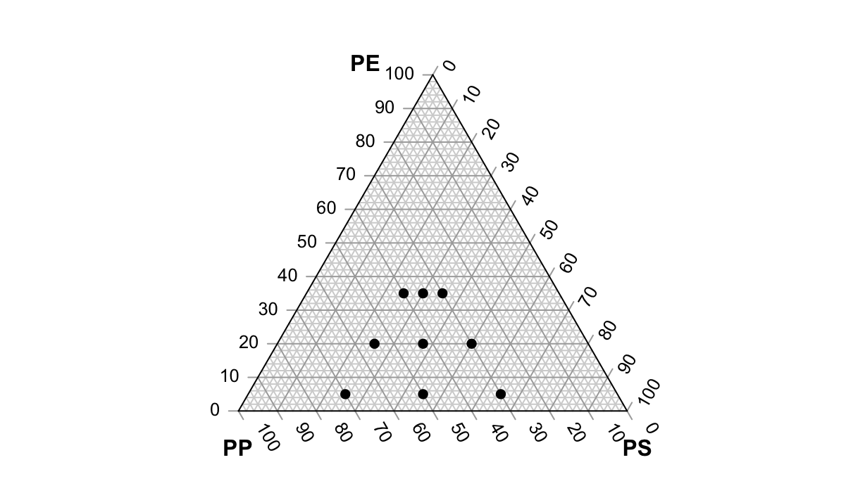
Let’s use the same regression as in the previous section to fake some data on this sub-domain, replicating twice each treatment:
df2 <- df %>%
  uncount(2, .id="rep") %>%
  select(-dimen) %>%
  mutate(failure=failure(x1, x2, x3) + rnorm(n(), sd=0.1))
Let’s build the model:
lm(failure~x1*x2*x3-1, data=df2) %>% summary()
Call:
lm(formula = failure ~ x1 * x2 * x3 - 1, data = df2)

Residuals:
      Min        1Q    Median        3Q       Max
-0.108956 -0.058915  0.003325  0.050258  0.104542

Coefficients:
         Estimate Std. Error t value Pr(>|t|)
x1        13.0219     2.9283   4.447 0.000984 ***
x2         9.5903     0.6711  14.290 1.90e-08 ***
x3        16.1321     0.5357  30.116 6.39e-12 ***
x1:x2     19.4790    10.4108   1.871 0.088161 .
x1:x3     -1.2769     8.9057  -0.143 0.888587
x2:x3      3.4179     2.7320   1.251 0.236871
x1:x2:x3 -14.2064    30.8291  -0.461 0.653911
---
Signif. codes:  0 '***' 0.001 '**' 0.01 '*' 0.05 '.' 0.1 ' ' 1

Residual standard error: 0.0816 on 11 degrees of freedom
Multiple R-squared:      1, Adjusted R-squared:      1
F-statistic: 8.052e+04 on 7 and 11 DF,  p-value: < 2.2e-16
df2.lm <- lm(failure~x1+x2+x3+ x1:x2 - 1, data=df2)
df2.lm %>% summary()
Call:
lm(formula = failure ~ x1 + x2 + x3 + x1:x2 - 1, data = df2)

Residuals:
      Min        1Q    Median        3Q       Max
-0.104271 -0.081257  0.000122  0.045705  0.163857

Coefficients:
      Estimate Std. Error t value Pr(>|t|)
x1     11.4718     0.6334  18.112 4.10e-11 ***
x2     10.4476     0.1827  57.172  < 2e-16 ***
x3     16.5531     0.1317 125.704  < 2e-16 ***
x1:x2  17.4749     2.1186   8.248 9.58e-07 ***
---
Signif. codes:  0 '***' 0.001 '**' 0.01 '*' 0.05 '.' 0.1 ' ' 1

Residual standard error: 0.09832 on 14 degrees of freedom
Multiple R-squared:      1, Adjusted R-squared:      1
F-statistic: 9.707e+04 on 4 and 14 DF,  p-value: < 2.2e-16
failure <- function(a, b, c) predict(df2.lm, newdata=data.frame(x1=a, x2=b, x3=c))With this function we can create the plot, but before we have to define a list of corners of the subset domain, in order to restrict the plot:
subdomain <- list(
  c(5, 25, 70)/100,
  c(35, 25, 40)/100,
  c(35, 35, 30)/100,
  c(5, 65, 30)/100
)
Now we can do the contour plot:
par(mar=rep(0, 4))
TernaryPlot(atip="A", btip="B", ctip="C", grid.minor.lines = 1, region=subdomain)
TernaryContour(failure, filled=T)
TernaryPoints(df %>% select(x1:x3), cex=scales::rescale(df$y, to=c(0.5, 2)), pch=16)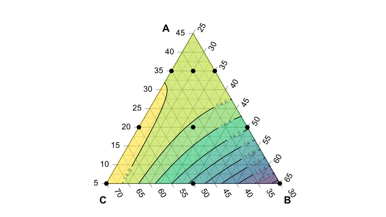
That’s all, folks!