ggpoints <- list(
  geom_point(size=0.5),
  coord_equal(xlim=c(-5, 25), ylim=c(-5,15))
)

set.seed(0)
N <- 1000
tibble(
  x = rnorm(N, mu_x, sigma_x),
  y = rnorm(N, mu_y, sigma_y)
) %>%
  ggplot(aes(x = x, y = y)) +
  ggpoints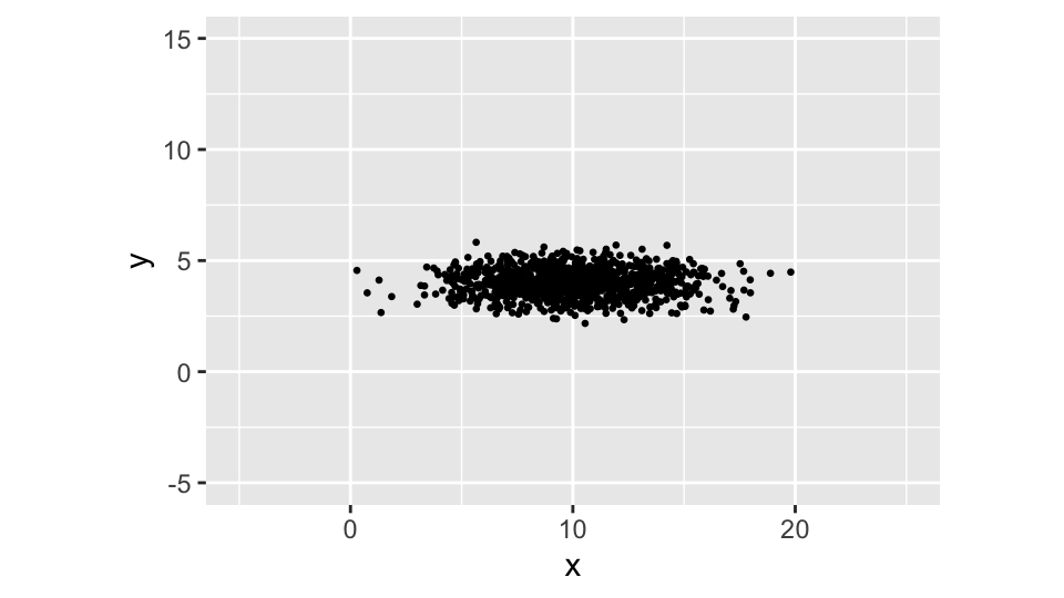
Paolo Bosetti
2024-Oct-30
Multivariate distributions are the multi-dimensional equivalent to common distributions. The univariate normal distribution \(\mathcal{N}(\mu, \sigma)\), for example, has a multivariate counterpart, the multivariate normal distribution \(\mathcal{N}(\boldsymbol{\mu}, \boldsymbol{\Sigma})\). The latter is characterized by a vector of means \(\boldsymbol{\mu}\) and a covariance matrix \(\boldsymbol{\Sigma}\). In the bivariate case, its density function is a “hat” shaped surface, with the peak at the mean vector \(\boldsymbol{\mu}\) and the axes of the hat aligned with the eigenvectors of the covariance matrix \(\boldsymbol{\Sigma}\).
Note that we’re denoting the covariance matrix as \(\boldsymbol{\Sigma}\) and not as \(\boldsymbol{\Sigma}^2\) as we would do for the variance. This is because the covariance matrix is a matrix, not a scalar.
We are going to see how to generate a multivariate distribution with given parameters and the opposite: how to estimate the parameters of a multivariate distribution from a cloud of points.
Suppose that we have two non-correlated random variables \(x\) and \(y\) with means \(\mu_x <- 10\) and \(\mu_y = 4\) and standard deviations \(\sigma_x = 3\) and \(\sigma_y <- 0.6\). The covariance between \(x\) and \(y\) — since these are independent — is obviously zero.
We are here forcing both axes to have the same scale, so that the cloud of points is not distorted and we can easily estimate the angles.
ggpoints <- list(
geom_point(size=0.5),
coord_equal(xlim=c(-5, 25), ylim=c(-5,15))
)
set.seed(0)
N <- 1000
tibble(
x = rnorm(N, mu_x, sigma_x),
y = rnorm(N, mu_y, sigma_y)
) %>%
ggplot(aes(x = x, y = y)) +
ggpoints
Being the two variables independent, the scatter plot shows a cloud of points with elliptical shape that — regardless the values we pick for the means and variances — is always aligned with the axes of the plot (or round, if the two variances are equal).
But what if we introduce a correlation between the two variables?
N <- 1000
tibble(
  x = rnorm(N, mu_x, sigma_x),
  y = x + rnorm(N, mu_y/5-5, sigma_y)
) %>%
  ggplot(aes(x = x, y = y)) +
ggpoints 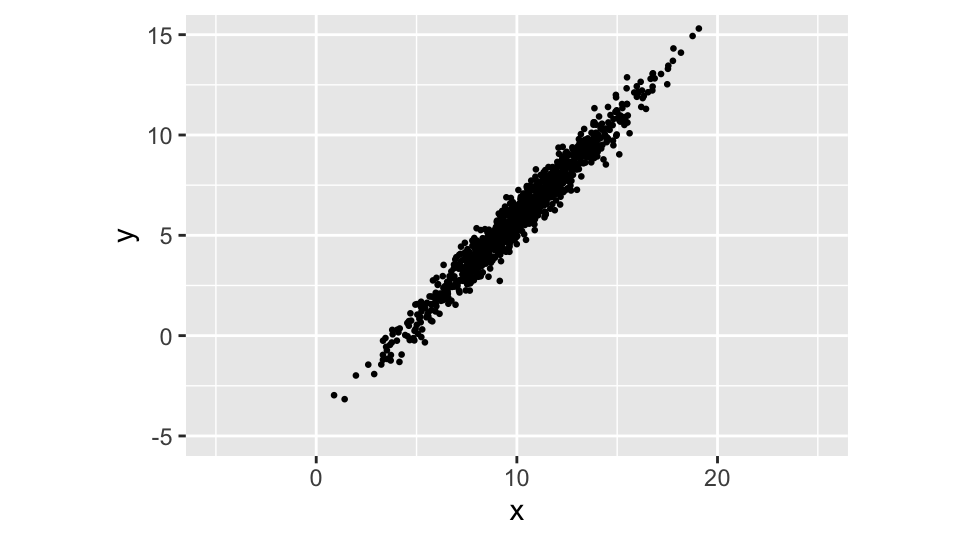
Now the cloud is roughly aligned with the line \(y = x\), because we introduced a correlation between the two variables. The correlation is positive, because the cloud is tilted to the right.
This is the visible aspect of covariance. In bivariate distributions, the means vector \(\boldsymbol{\mu}\) is the center of the cloud, while the covariance \(\boldsymbol{\Sigma}\) is a matrix, for to represent the distribution alignment and shape we need a \(2\times 2\) matrix, whose eigenvalues and eigenvectors determine the shape (the main axes) and the orientation (the alignment vectors) of the cloud.
Rather than defining the relationship between the two variables when generating the random values, we can define it in terms of the covariance matrix \(\boldsymbol{\Sigma}\), using the MASS::mvrnorm() function:
data <- mvrnorm(
  n = N,
  mu = c(mu_x, mu_y),
  Sigma = matrix(c(5.5, 4.5, 4.5, 5.5), nrow = 2)
)
colnames(data) <- c("x", "y")

data %>%
  ggplot(aes(x = x, y = y)) +
  ggpoints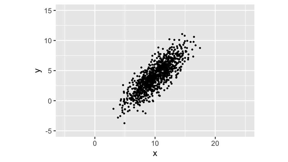
Now if we want to control the inclination angle of the cloud, we can change the covariance matrix. It’s easy to build a function to generate the covariance matrix \(\boldsymbol{\Sigma}\) from the vector of main variances and the list directional vectors (we’re not checking for orthogonality, though!):
In 2D, the two directional vectors can be calculated from the desired nominal angle \(\vartheta_n\):
theta_n <- 15 / 180 * pi
cm_in <- covmat(
  c(sigma_x^2, sigma_y^2), # main components
  list(     # directional vectors
    c(cos(theta_n), sin(theta_n)),
    c(cos(theta_n+pi/2), sin(theta_n+pi/2))
  )
)
cat("Covariance matrix in:\n")
Covariance matrix in: [,1] [,2]
[1,] 8.42123 2.1600000
[2,] 2.16000 0.9387703So now we can generate a cloud of points with the desired inclination angle and plot it:
So we’re now able to generate a multivariate distribution with given parameters as position (\(\boldsymbol{\mu}\)), principal component standard deviations (eigenvalues of \(\boldsymbol{\Sigma}\)) and inclination direction (eigenvectors of \(\boldsymbol{\Sigma}\)).
Now let’s go backwards: given a cloud of points, how can we estimate the principal components and alignment of the covariance matrix?
The covariance matrix can be calculated in R with the usual cov() function, and its eigenvectors and eigenvalues can be calculated with the eigen() function. The main eigenvector is the one corresponding to the largest eigenvalue, and the angle of the cloud is the angle of this vector with the \(x\) axis.
Covariance matrix:
 7.986343 1.994013 1.994013 0.8686458
Eigenvalues:
 8.506893 0.348096
Principal Eigenvector:
 -0.9675731 -0.2525911
Principal standard deviations:
 2.916658 0.5899966
alpha <- atan2(ev1[2], ev1[1])
if (alpha < 0) alpha <- alpha + pi
cat("\nAngle:\n", alpha / pi * 180)
Angle:
 14.6309
In particular, compare the principal standard deviations with the nominal ones (3 and 0.6), and the angle with the nominal one (15).
Now we can plot the cloud of points together with the ellipsis representing the prediction area, say at 3 standard deviations from the center. The slope and intercept of the main axis can be calculated from the main eigenvector:
Slope:
 0.2610564
Intercept:
 1.363394
The lengths of the main and secondary axes of the ellipsis are the square roots of the eigenvalues, multiplied by 3:
Main and secondary axes lengths:
 8.749974 1.76999
Now we can plot the cloud of points, the main axis and the ellipsis. As we see, the angle is pretty close to the nominal one:
data %>%
  ggplot(aes(x=x, y=y)) +
  ggpoints +
  geom_abline(intercept=b, slope=a, color="red") +
  geom_ellipse(aes(x0=mean(x), y0=mean(y), a=cmd[1], b=cmd[2], angle=alpha), color="blue") +
labs(title=paste0("Angle: ", round(alpha * 180/pi, 2), "°")) 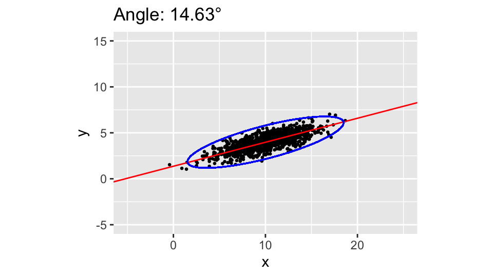
That’s all, folks!