Rationale

In this post we will show how to cluster a dataset using the DBSCAN algorithm. We will use the dbscan package, which is a very efficient implementation of the algorithm.

Building on top of the last post, we will generate a dataset with several multi-variate normal samples, cluster it using DBSCAN, and eventually identify the position and shape of the clusters ellipsoids.

As a bonus, we’re going to use some handy purrr mapping functions, as imap and reduce.

Data generation

We are re-using the covmat() function that we defined here.

First of all, we create a list of parameters, one element per cluster, each cluster with information about number of points, position (means) and orientation:

params <- list(
  list(N=1000, mx=10, my=4, s1=3, s2=1, theta=15),
  list(N=100, mx=2, my=6, s1=1, s2=0.2, theta=30),
  list(N=200, mx=4, my=1, s1=2, s2=0.5, theta=-60)
)

Then we modify this list to include the covariance matrix, and the cluster index:

Note the use of list_assign to add the new elements to the list within the imap function. This operates on each iterated element by reference.

set.seed(0)
params <- imap(params, \(e, i) {
  theta <- e$theta * pi / 180
  cm <- covmat(
    c(e$s1^2, e$s2^2),
    list(
      c(cos(theta), sin(theta)),
      c(cos(theta+pi/2), sin(theta+pi/2))
    )
  )
  list_assign(e, i=i, cm = cm)
  }
)

Now we can use reduce() to create a data array with mvrnorm() and merge all the data into a single tibble:

df <- params %>% 
  reduce(
    \(tbl, e) {
      cm <- mvrnorm(e$N, c(e$mx, e$my), e$cm)
      colnames(cm) <- c("x", "y")
      bind_rows(tbl, cm %>% as_tibble() %>% mutate(group=e$i))
    },
    .init = tibble()
  ) %>% 
  mutate(group = as.factor(group))

df %>% 
  ggplot(aes(x, y, color=group)) +
  geom_point(size=0.5)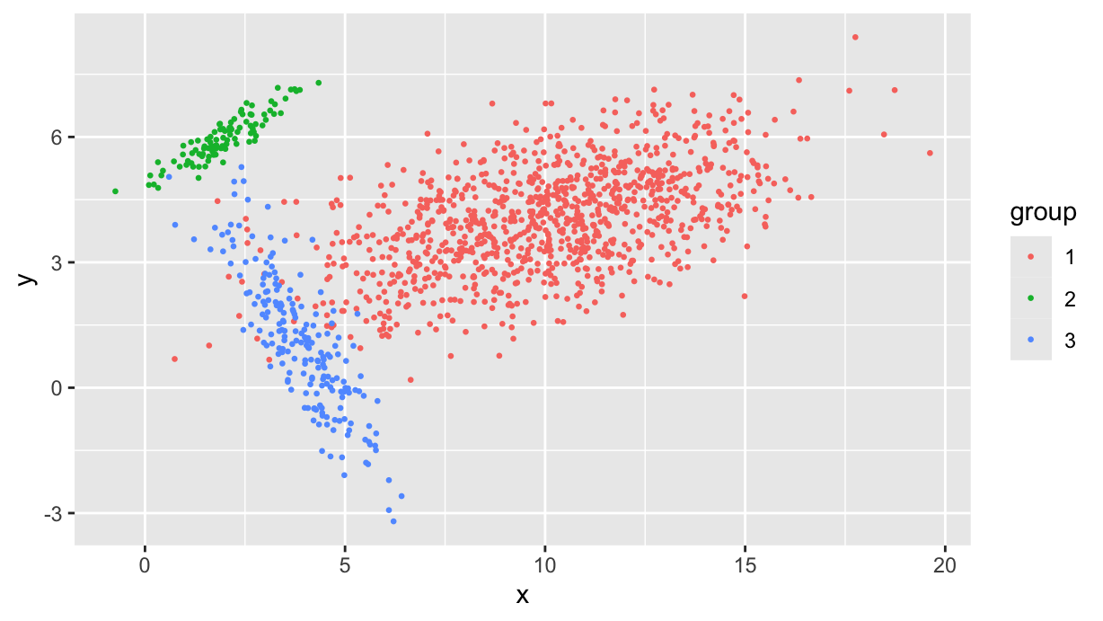

Now we want to cluster this dataset in df, obtaining position and orientation of the three clusters.

Clustering

The DBSCAN algorithm uses a distance threshold eps and a minimum number of points minPts to define clusters. A clever way to choose these parameters is to use the kNNdist() function from the dbscan package:

Note that the MASS package overrides the select() function from dplyr, so we need to use dplyr::select() to avoid conflicts. Also, we are using kNNdist() rather than kNNdistplot() to get the data in a tibble and then make a ggplot.

k <- 10
tibble(
  dist = kNNdist(as.matrix(df %>% dplyr::select(x, y)), k=k),
  i = seq_along(dist)
) %>% 
  mutate(dist = dist %>% sort() %>% as.numeric()) %>% 
  ggplot(aes(x=i, y=dist)) +
  geom_line() + 
  labs(x="Sorted point index", y=paste0(k, "-kNN distance")) +
  scale_y_log10(breaks=c(seq(0, 1, 0.1), seq(1, 10, 1)))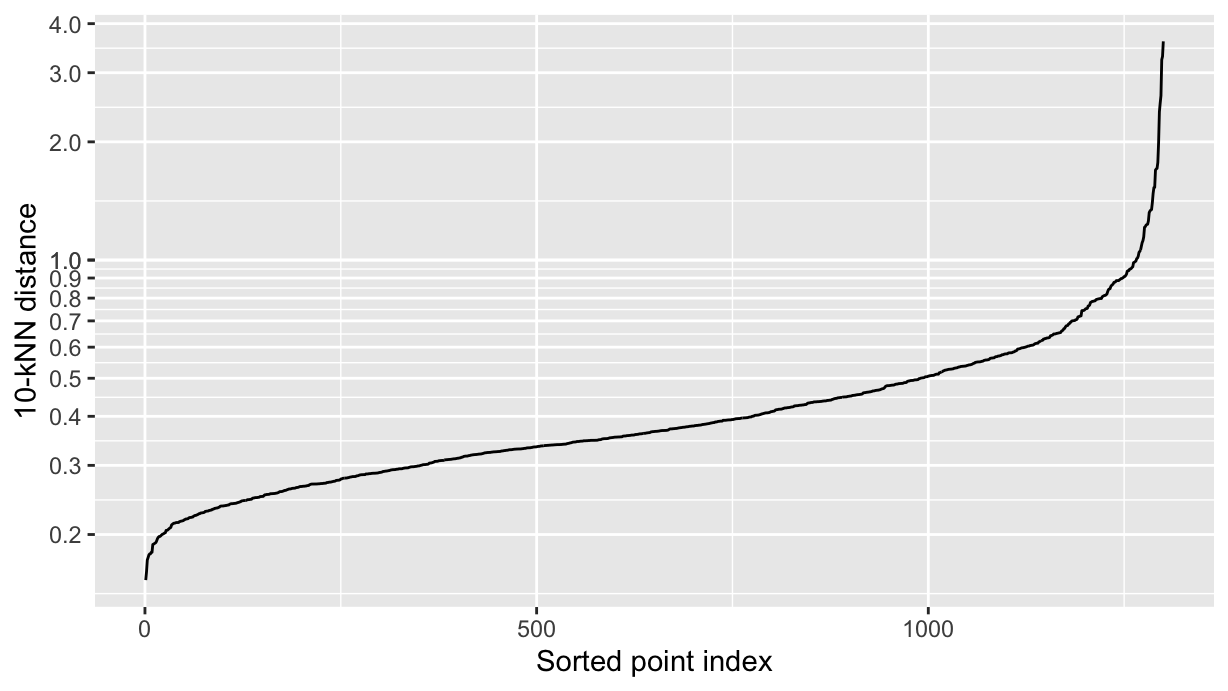

We want to use for the eps parameter the distance at the knee of the curve, which is around 0.48 in this case. We can now cluster the dataset, where each cluster has a minimum of 10 points:

df <- df %>% 
  mutate(
    cluster = as.factor(
      dbscan(dplyr::select(., x, y), eps=0.48, minPts=k)$cluster
    )
  )
  

df %>% 
  ggplot(aes(x, y, color=cluster, shape=group, alpha = cluster == 0)) +
  scale_alpha_manual(values=c(1, 1/3)) +
  geom_point(size=1) +
  guides(alpha="none")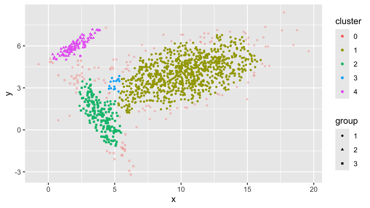

Note that the cluster 0 collects noise, i.e. points that are not part of any cluster.

Identification

First of all, we clean up the dataset by removing the noise points and the clusters with less than 20 points:

df.f <- df %>% 
  group_by(cluster) %>% 
  filter(cluster != 0, n() > 20) 

df.f %>% 
  ggplot(aes(x, y, color=cluster)) +
  geom_point(size=1)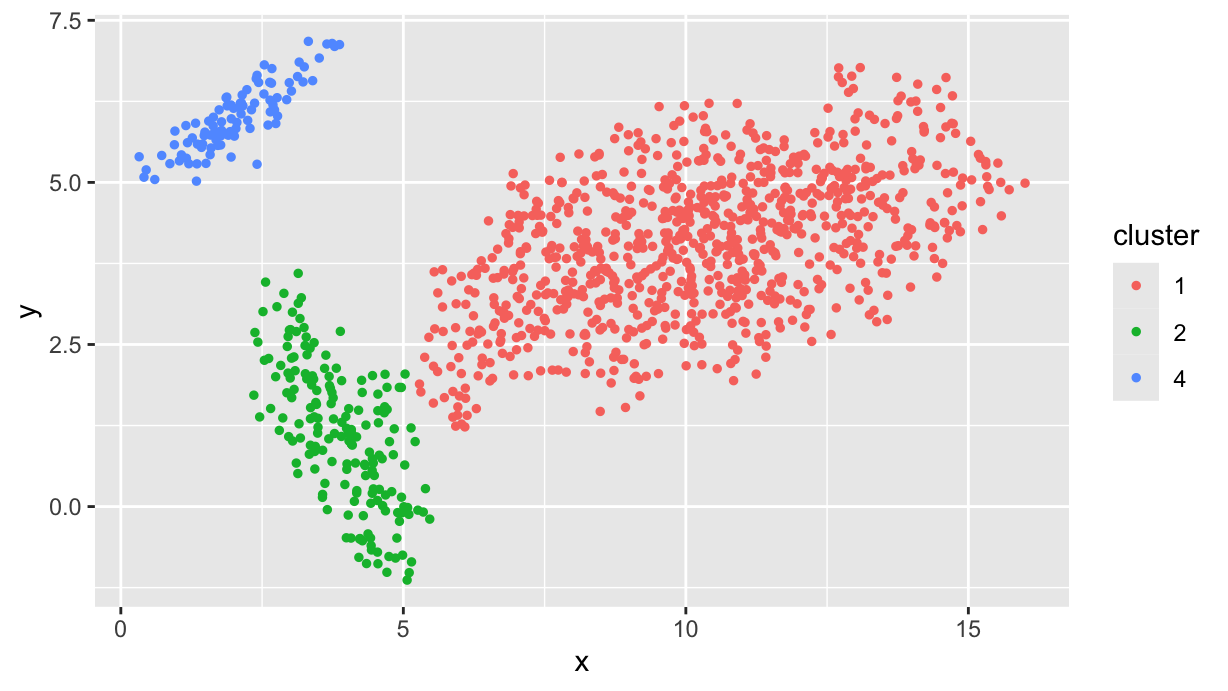

Now we create a function that takes a matrix or data frame with the two columns x and y and returns the parameters of the cluster:

calc_params <- function(data) {
  head(data)
  cm <- data %>% cov()
  cm.e <- eigen(cm)
  ev1 <- cm.e$vectors[,which.max(cm.e$values)]
  alpha <- atan2(ev1[2], ev1[1])
  if (alpha < 0) alpha <- alpha + pi
  sigma <- sqrt(cm.e$values)
  names(sigma) <- c("sigma1", "sigma2")
  list(
    mx = mean(data$x),
    my = mean(data$y),
    sigma = sigma,
    angle = alpha
  )
}

So we can apply this function to each cluster. Since df.f is grouped already, we just use reframe() to add a list column with the results of calc_params(), and then use unnest_wider() to expand this list into columns:

df.p <- df.f %>% 
  reframe(params = list(calc_params(tibble(x, y)))) %>% 
  unnest_wider(params) %>% 
  unnest_wider(sigma) %>% 
  mutate(angle_deg = angle * 180 / pi)

df.p %>% knitr::kable(digits=2)

cluster	mx	my	sigma1	sigma2	angle	angle_deg
1	10.27	4.06	2.51	0.91	0.27	15.35
2	3.92	1.10	1.22	0.51	2.10	120.40
4	2.04	6.01	0.91	0.22	0.55	31.74

We are almost there: now we have to plot the clustered points and the ellipses representing the clusters:

df.p %>% 
  ggplot() +
  geom_point(data=df.f, aes(x=x, y=y, color=cluster), alpha=1/3) +
  geom_ellipse(
    aes(x0=mx, y0=my, a=sigma1, b=sigma2, angle=angle, fill=cluster), 
    alpha=1/3)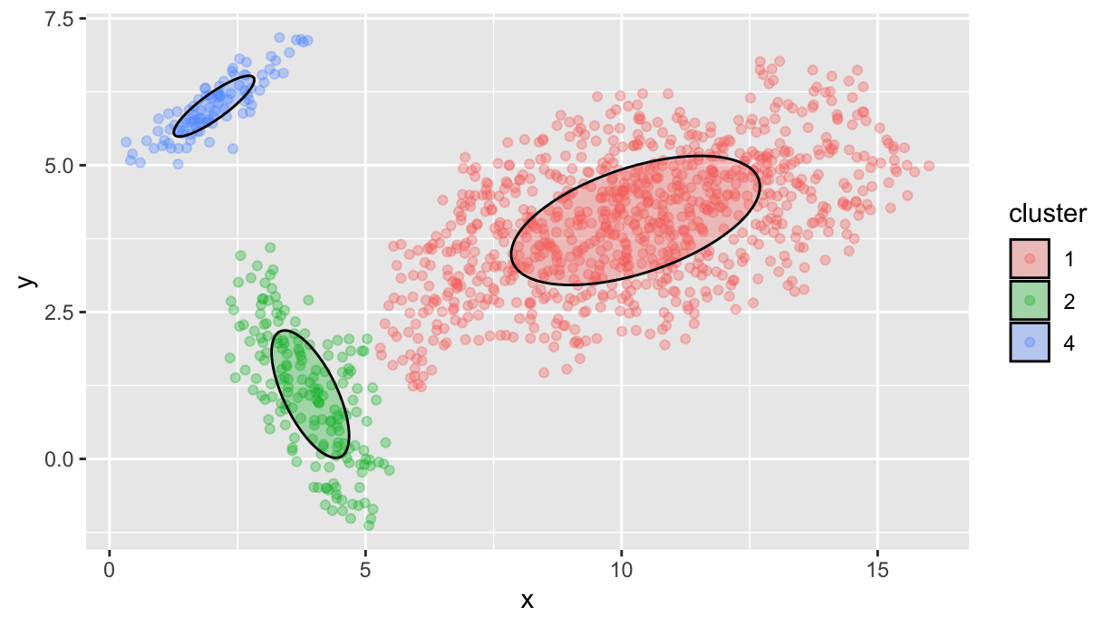

Finally, let’s compare with the initial parameters that we used for generating the data:

params %>% 
  reduce(
    \(tbl, e) tbl <- bind_rows(
      tbl, 
      c(x0=e$mx, y0=e$my, a=e$s1, b=e$s2, theta=e$theta)),
    .init = tibble()
  ) %>% 
  mutate(angle=theta / 180 * pi) %>% 
  ggplot() +
  geom_point(data=df.f, aes(x=x, y=y, color=cluster), alpha=0.1) +
  geom_ellipse(aes(x0=x0, y0=y0, a=a, b=b, angle=angle), linetype=2) +
  geom_ellipse(
    data=df.p, 
    mapping=aes(x0=mx, y0=my, a=sigma1, b=sigma2, angle=angle, fill=cluster), 
    alpha=1/3)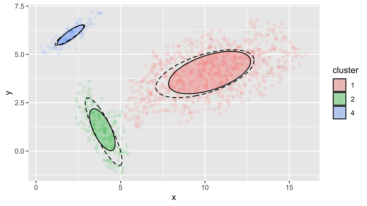

As we see, position and angles are generally well estimated, but the ellipses are typically smaller than the original ones. This is due to the fact that the DBSCAN algorithm is not able to capture the full extent of the clusters, but only the densest part of them (and the eps parameter affects how dense is that densest part).

That’s all, folks!