Recurring Satistics

Rationale

This memo reports the calculation scheme that can be adopted for calculating sample mean and variance statistics by using a pair of recurrence formulas. This approach comes handy whenever you have to perform a continuous, inline assessment of those indicators with minimum memory footprint (e.g. on microcontrollers), without the need of storing the whole set of sample values.

This is an easy one: given the stochastic variable \(x\) and by indicating its sample mean for a set of \(i\) observations as \(\bar x_i\), we have: \[\begin{eqnarray} \bar x_1 :=& x_1 \\ \bar x_n =& \frac{1}{n}\sum_{i=1}^{n} x_i \\ =& \frac{n-1}{n} \left(\sum_{i=1}^{n-1}\frac{x_i}{n-1}\right) + \frac{x_n}{n} \\ =& \frac{1}{n}\left((n-1) \bar x_{n-1} + x_n\right) \end{eqnarray}\] where \(x_n\) is the current observation (after \(n\) events), and \(x_1\) is the very first observation.

By using the last equation for \(\bar x_n\), the sample mean value \(\bar x_n\) can be continuously updated at every acquisition using only the last observation \(x_n\), the previous value of the sample mean \(\bar x_{n-1}\), and the total number of observations \(n\). There is no need for storing the whole set of observations, and the algorithm complexity is \(O(1)\).

Sample variance

The recurrence formula for sample variance is a little more complex, and care must be payed in the formulation in order to avoid differences between small quantities, which may bring to large rounding errors.

By definition of sample variance for \(n\) observations, \(s_n^2\): \[\begin{align} s_n^2 =& \sum_{i=1}^{n}\frac{(\bar x_n - x_i)^2}{n-1} = \frac{SS_n}{n-1} \\ =& \frac{1}{n-1}\sum_{i=1}^{n}\left(x_i^2 - 2x_i\bar x + \bar x^2\right) \\ =& \frac{1}{n-1}\left(\sum_{i=1}^{n}x_i^2 - \bar x^2\right) \\ s_n =& \sqrt{\frac{1}{n-1}\left(\sum_{i=1}^{n}x_i^2 - \frac{1}{n}\left(\sum_{i=1}^{n} x_i\right)^2\right)} \end{align}\]

The sum of squares \(SS_n\) (which is the only part in the definition of sample variance that is depending on previous values) can be thus be expressed as: \[\begin{align} SS_n = \left(\sum_{i=1}^{n}x_i^2 - \frac{1}{n}\left(\sum_{i=1}^{n} x_i\right)^2\right) \end{align}\] so that the increment in sum of squares can be obtained: \[\begin{align} SS_n - SS_{n-1} &= \sum_{1=1}^n x_i^2 - \frac{1}{n}\left(\sum_{1=1}^n x_i\right)^2 - \sum_{1=1}^{n-1} x_i^2 + \frac{1}{n-1}\left(\sum_{1=1}^{n-1} x_i\right)^2 \end{align}\] where we can substitute: \[\begin{align} \sum_{1=1}^n x_i &= n \bar x_n \\ \sum_{1=1}^{n-1} x_i &= \sum_{1=1}^n x_i - x_n = n \bar x_n - x_n \\ \sum_{1=1}^{n} x_i^2 - \sum_{1=1}^{n-1} x_i^2 &= x_n^2 \end{align}\] thus having: \[\begin{align} SS_n - SS_{n-1} &= x_n^2 - \frac{1}{n}(n \bar x_n)^2 + \frac{1}{n-1}(n \bar x_n -x_n)^2 \\ &= x_n^2 - n\bar x_n^2 + \frac{1}{n-1}(n^2 \bar x_n^2 - 2n \bar x_n x_n + x_n^2) \\ &= \frac{1}{n-1}(n x_n^2 + n \bar x_n^2 - 2 n \bar x_n x_n) \\ &= \frac{n}{n-1}(\bar x_n - x_n)^2 \end{align}\] after which we have the recurrence formula for the sum of squares: \[\begin{align} SS_n &= SS_{n-1} + \frac{n}{n-1}(\bar x_n - x_n)^2 \end{align}\]

Accordingly, the recurrence formula for the sample standard deviation (square root of variance) is: \[\begin{align} s_1 &:= 0 \\ s_n &= \sqrt{\frac{1}{n-1} \left( (n-2) s_{n-1}^2 + \frac{n}{n-1}(\bar x_n - x_n)^2 \right)} \end{align}\]

In conclusion, a typical pseudocode for running calculation of \(\bar x\) and \(s\) indicators is as follows:

\begin{algorithmic} \Require $\mathtt{read\_value}()$: returns a new observation of $x$ at each call \State $\bar x \gets \mathtt{read\_value}()$ \Comment{Initializations} \State $s \gets 0$ \State $n \gets 1$ \Repeat \Comment{Main loop} \State $n \gets n+1$ \State $x \gets \mathtt{read\_value}()$ \State $\bar x \gets \frac{1}{n}\left((n-1) \bar x + x\right)$ \Comment{Update sample mean} \State $s \gets \sqrt{\frac{1}{n-1} \left( (n-2) s^2 + \frac{n}{n-1}(\bar x - x)^2\right)}$ \Comment{Update sample std.~dev.} \State Perform operations on $\bar x$ and $s$ \Until{exit condition is true} \end{algorithmic}

R implementation

The following R code implements the above pseudocode, with some care to make it fun to use and pipe-ready:

rstats <- function(prev, x=NULL, echo=FALSE) {
  result <- list(mean=NA, sd=0, n=0)
  if (!is.list(prev)) {
    v <- prev
    result$mean <- v
    result$n <- 1
  } else {
    n <- prev$n + 1
    m <- 1/n * ((n-1) * prev$mean + x)
    s <- ifelse(n > 1, sqrt(1/(n-1) * ((n-2) * prev$sd^2 + n/(n-1) * (m - x)^2)), 0)
    result$mean <- m
    result$sd <- s
    result$n <- n
  }
  if (echo)
    cat(sprintf("n: %d, mean: %.2f, sd: %.2f\n", 
                result$n, result$mean, result$sd))
  invisible(result)
}

Simple use:

rstats(10) %>% rstats(11) %>% rstats(12, echo=T)

n: 3, mean: 11.00, sd: 1.00

To be compared with:

v <- 10:12
cat(sprintf("mean: %.2f, sd: %.2f, n: %d\n", mean(v), sd(v), length(v)))

mean: 11.00, sd: 1.00, n: 3

Thanks to how we built the rstats function, we can use it in a dplyr pipeline using purrr::accumulate():

set.seed(0)
df <- tibble(
  i=1:100, 
  x=rnorm(100, mean=10, sd=2)
) %>% 
  mutate(
    # Warn: the first element of the list is the initial value of the 
    # accumulator
    # This creates a list column with the stats at each step
    stats=accumulate(
      x, 
      ~ rstats(.x, .y), 
      .init=list(mean=first(x), sd=0, n=0))[2:(n()+1)],
    # usual cumulative stats:
    mean = cummean(x),
    sd = imap_dbl(x, ~ sd(x[1:.y]))
  ) %>% 
  # unnest the list column
  hoist(stats, rmean=1, rsd=2) %>% 
  mutate(
    mean = mean - rmean, 
    sd = sd - rsd
  ) %>% 
  pivot_longer(cols=c(mean, sd), names_to="statistic", values_to="difference") 

df %>% 
  ggplot(aes(x=i, y=difference)) +
  geom_line(aes(color=statistic))

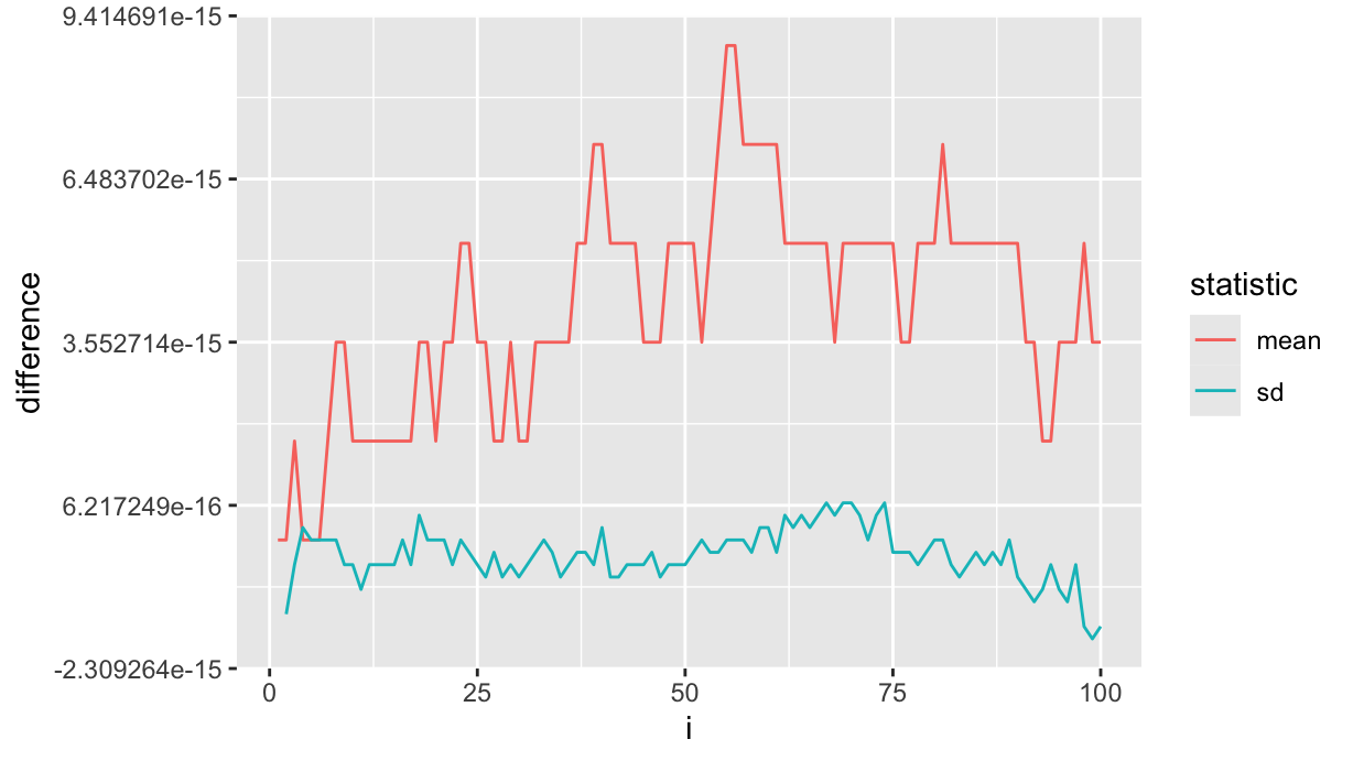
So the recursion formulas do suffer from numerical precision, but the difference is not that big.

Cpp implementation

Much more interesting is the C/C++ implementation of the same algorithm. The following code is a simple, pure C implementation, plus a Rcpp wrapper to make it available in R with an interface similar to the R version:

#include "Rcpp.h"
using namespace Rcpp;


// Pure C version. n, mean and sd are IN/OUT parameters:
void rstats_c(double x, unsigned long int *n, double *mean, double *sd) {
  if (*n == 0) {
    *mean = x;
    *sd = 0;
    *n += 1;
  } else {
    *n += 1;
    double m = 1.0/ *n * ((*n-1) * (*mean) + x);
    double s = sqrt(1.0/(*n-1.0) * ((*n-2) * pow(*sd, 2) + 
               *n/(*n-1.0) * pow(m - x, 2)));
    *mean = m;
    *sd = s;
  }
}

//[[Rcpp::export]]
List rstats(List &prev, double x) {
  double mean = prev["mean"];
  double sd = prev["sd"];
  unsigned long int n = prev["n"];
  rstats_c(x, &n, &mean, &sd);
  return List::create(
    Named("n") = n,
    Named("mean") = mean,
    Named("sd") = sd
  );
}

Now we can use the C++ version in R, paying attention that the C++ version interface is less smarter and it needs to have an initial zeroed list as input on the frst call:

rstats(list(mean = 0, sd=0, n=0), 10) %>% rstats(11) %>% rstats(12)

$n
[1] 3

$mean
[1] 11

$sd
[1] 1

That’s all, folks!