data <- read_csv("https://paolobosetti.quarto.pub/data/kfold.csv",
                 show_col_types = FALSE)
data %>% ggplot(aes(x=x, y=y)) + geom_point()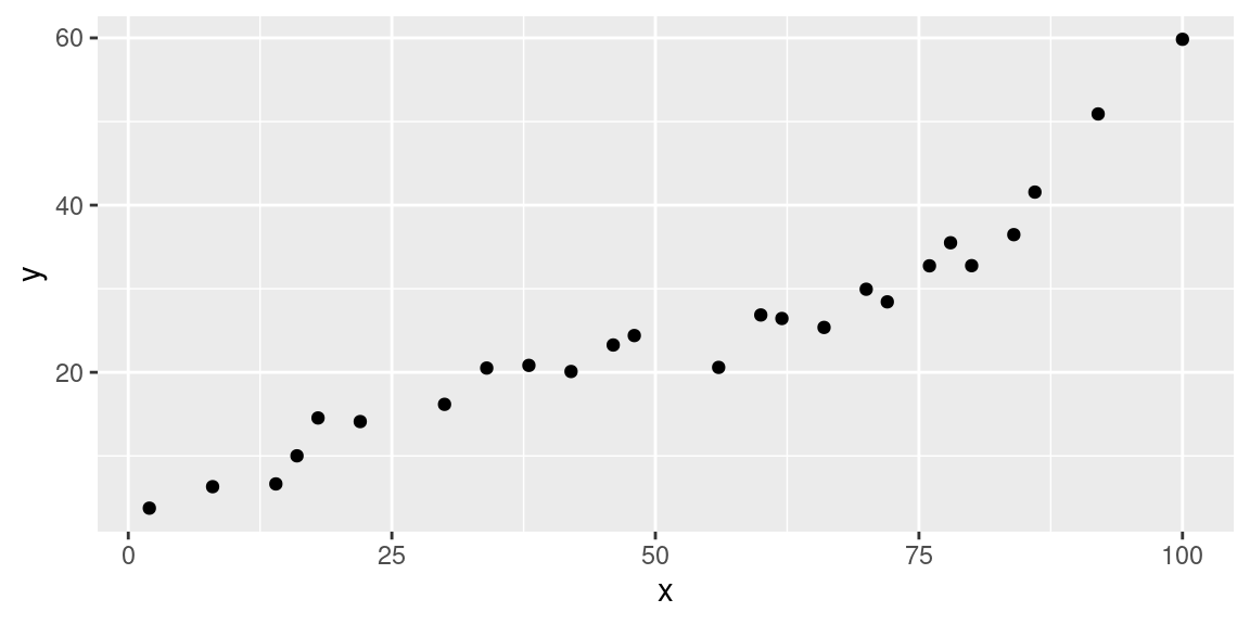
Paolo Bosetti
20250913
We load the data from a web address and make a quick plot:
The regression of a linear model is performed with the lm() function. It takes two arguments:
The formula is expressed in the formula notation, which is a map from an analytical regression model, as \(y_i = a + bx_i + cx_i^2 + \varepsilon_i\) to a formula object as y~x + I(x^2)
To build a formula from a model you typically:
I()y~x1 + x2, which corresponds to \(y_i = a + bx_{1,i} + cx_{2,1} + \varepsilon_i\) or as y~x1 + x2 + x1:x2, which corresponds to \(y_i = a + bx_{1,i} + cx_{2,1} + dx_{1,i}x_{2,i} +\varepsilon_i\)y~x1 + x2 + x1:x2 can be abbreviated as y~x1*x2y~x + I(x^2) - 1So let’s build a linear model of degree 2:
data.lm <-lm(y~x, data=data)

data %>%
  add_predictions(data.lm) %>%
  ggplot(aes(x=x)) +
  geom_point(aes(y=y)) +
  geom_line(aes(y=pred))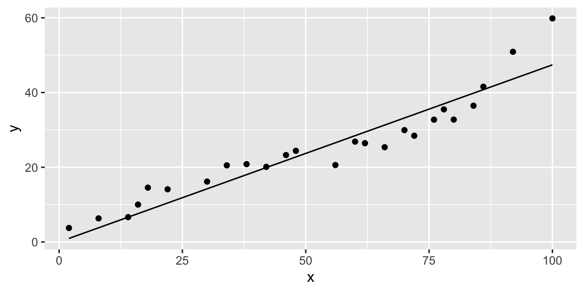
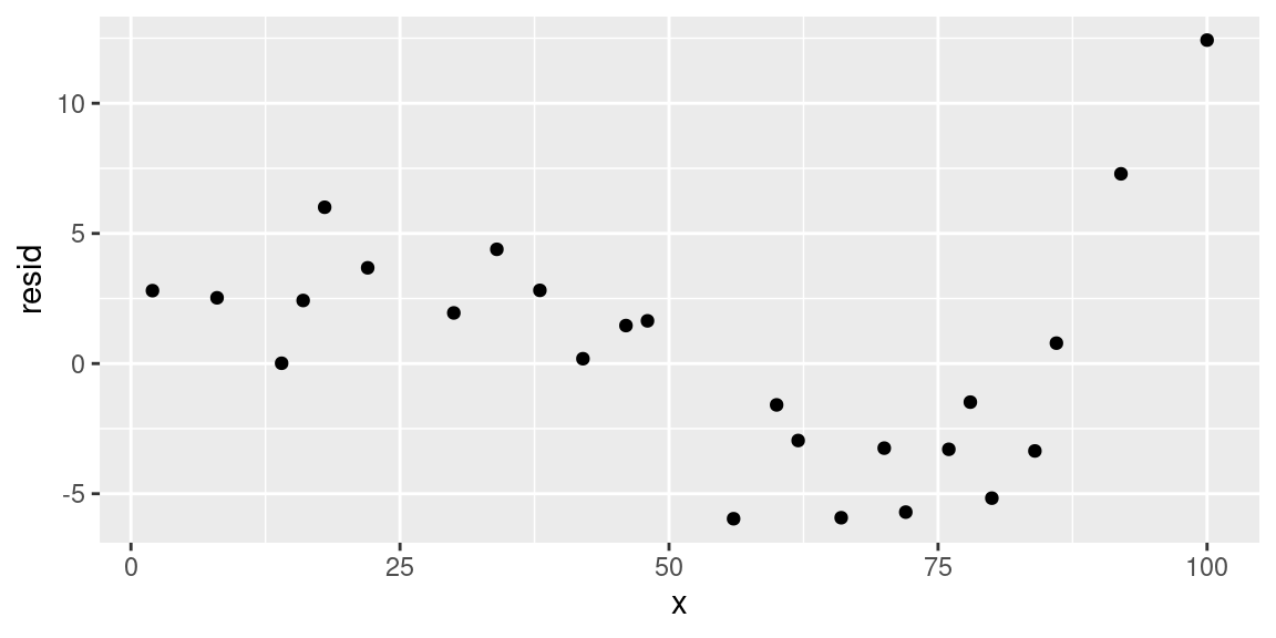
We note that the residuals show a rather strong pattern, meaning that the linear relationship is underfitting the data, and thus we need to increase the degree of the fitting polynomial. But how much so?
The degree of the fitting polynomial is a hyper-parameter. In fact, regression parameters are the coefficients of the polynomial, to be calculated typically by minimizing the root mean square of the residuals. But the degree of the polynomial is a parameter that defines the number of regression parameters, and that is why it is named a hyper-parameter. Identifying the best hyper-parameter(s) is the aim of validation and cross-validation strategies.
In our case we want to compare polynomial fits up to degree 12, using a map:
Quality of a regression can be verified with different metrics:
Typically, the root means square of error (RMSE) and the mean absolute error (MAE) are the most commonly used metrics.
Let’s see how the RMSE and the \(R^2\) metrics change when the polynomial degree increases. To do that we build a table with three columns:
We extract these data from the list of linear models above created, fits. For each fitted linear model (an entry in fits), the \(R^2\) and RMSE can be extracted with the functions rsquare() and rmse(), respectively.
We use map_dbl() to map these functions over the list of polynomial degrees. The resulting table is then used to make a plot:
tibble(
  degree=1:12, # deg starts from 2!
  rsquare=fits %>% map_dbl(~rsquare(., df)),
  rmse=fits %>% map_dbl(~rmse(., df))
) %>%
  pivot_longer(-degree, names_to = "Index") %>%
  ggplot(aes(x=degree, y=value)) +
  geom_line() +
  facet_wrap(~Index, nrow=2, scales="free")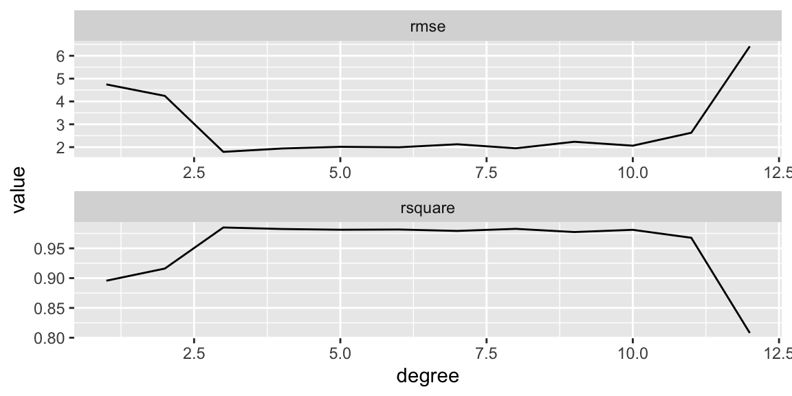
The \(R^2\) increases pretty quickly and saturates after degree 3. The RMSE decreases sharply and monotonically. It’s hard to figure out the point where over-fitting starts.
To solve the problem we use K-fold cross validation. It is a regression strategy where we split the dataset into \(k\) subsets, or folds, with roughly the same amount of observations. Then:
In R, we use the caret library to simplify this process. The caret::train() function performs the folding for a given model: it takes as arguments the model formula, the regression function (in our case lm()), the dataset, and a list of parameters that can be created with the supporting trainControl() function.
The trainControl() function is used to define the details on the cross validation strategy to use. In our case we use the repeated K-fold cross validation, named "repeatedcv", which repeates a K-fold a given number of times.
In fact, the folds are defined by randomly sampling the initial dataset, so that the resulting RMSE (or any other metric) is also a random variable. Repeating the K-fold 100 times makes the whole process more robust:
ctrl <- trainControl(method = "repeatedcv", number=5, repeats=100)
model <- train(y~poly(x,8), data=data, method="lm", trControl=ctrl)

model
Linear Regression
25 samples
1 predictor
No pre-processing
Resampling: Cross-Validated (5 fold, repeated 100 times)
Summary of sample sizes: 20, 20, 21, 20, 19, 20, ...
Resampling results:
RMSE Rsquared MAE
10.3213 0.9241026 6.25129
Tuning parameter 'intercept' was held constant at a value of TRUEThe model object contains a field named model$results that is a table with all the available performance metrics:
| intercept | RMSE | Rsquared | MAE | RMSESD | RsquaredSD | MAESD |
|---|---|---|---|---|---|---|
| TRUE | 10.3213 | 0.9241026 | 6.25129 | 23.37541 | 0.1183862 | 12.14192 |
Now we want to repeat the K-fold validation over the list of formulas corresponding to the set of polynomials with degrees from 1 to 12. We use again the map() function:
Note the unnest() function at the end: the model field $results is actualy a table, so without that function in fit_quality we would get a column results that contains a list of tables. The unnest() function flattens this list of tables in place.
Now we can finally make a plot of the metrics as a function of the polynomial degree:
fit_quality %>%
  select(-intercept, -starts_with("Rsquared")) %>%
  pivot_longer(-degree, names_to = "metric") %>%
  ggplot(aes(x=degree, y=value, group=metric, color=metric)) +
  geom_line() +
  geom_point() +
  scale_y_log10() +
  scale_x_continuous(breaks=1:12)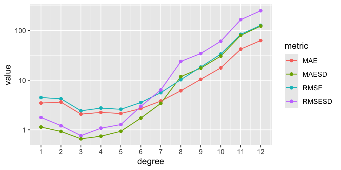
We observe that the minima of any metric happens at degree 3. This means that below that value we have underfitting, above we have overfitting (i.e. the model is loosing generality).
So we can finally accept the model \(y_i=a + bx_i + cx_i^2 + dx_i^3 + \varepsilon_i\) (a degree 3 polynomial in \(x_i\)):
data.lm <- lm(y~poly(x, 3), data=data)

data %>%
  add_predictions(data.lm) %>%
  ggplot(aes(x=x, y=y)) +
  geom_point() +
  geom_line(aes(y=pred))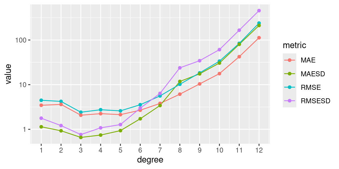
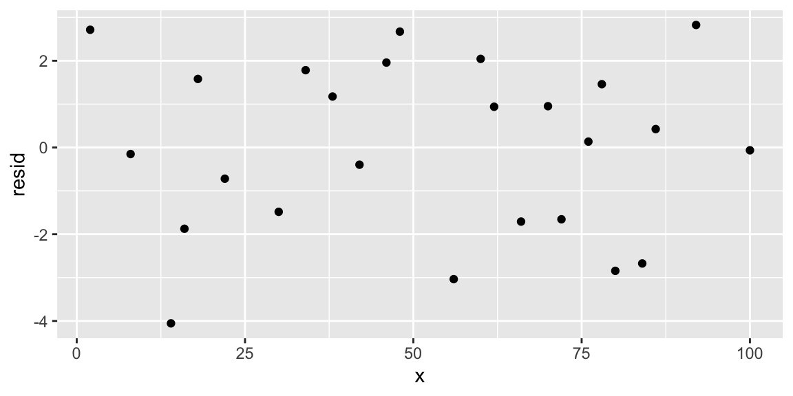
We confirm that the residuals are free from patterns. We can also plot a confidence interval of the same regression by using the geom_smooth() layer in a ggplot:
Paolo Bosetti Paolo Bosetti ADAS Contenuti /slides/ADAS/index.html Intro /slides/ADAS/0-intro.html Statistica /slides/ADAS/1-statistica.html Linguaggio R /slides/ADAS/2-R-intro.html Regressione /slides/ADAS/3-regressione.html Bootstrap /slides/ADAS/4-bootstrap.html Misura /slides/ADAS/5-misura.html Design of Experiments /slides/ADAS/6-DoE.html Serie temporali /slides/ADAS/7-serie_temporali.html DESAnED Table of Contents /slides/DESANED/index.html Statistics /slides/DESANED/1-statistics.html Intro to R language /slides/DESANED/2-R-intro.html Regression /slides/DESANED/3-regression.html K-Fold validation /slides/DESANED/4-kfold.html /slides/DESANED/5-DoE.html Example Data /data.html Blog /blog/index.html About /about.html This project on GitHub https://github.com/pbosetti/teaching_site
K-Fold Cross Validation – Paolo Bosetti K-Fold Cross Validation – Paolo Bosetti K-Fold Cross Validation – Paolo Bosetti Paolo Bosetti